


Theory only takes you so far. To really understand hyperparameter tuning, you have to watch a default model get beaten by a tuned one on the same data. This code-along does exactly that, end to end, using nothing but scikit-learn.
The setup is a marketing problem every retailer faces. Contacting a customer costs money, so you want to predict who will actually respond to a campaign and target them first. The dataset is simulated, 8,000 customers with a realistic 21.5% response rate, and the structure is planted on purpose: genuine drivers like email engagement, recency, loyalty, and discount size, plus a few nonlinear interactions that reward a model clever enough to find them. That last detail matters, because it is what gives tuning something real to discover.
The journey from default to tuned
The code-along follows the full project lifecycle, but the heart of it is the tuning, which climbs a ladder from crude to sophisticated.
It starts with a baseline: a Random Forest with default settings, which scores a test ROC-AUC of 0.693. That is the number to beat.
Then comes manual search, a simple loop over the tree depth with cross-validation, the most basic tuning there is. A learning curve over the number of trees turns that into a picture, showing exactly where adding more trees stops helping.
From there it automates. GridSearchCV exhaustively tests a small Random Forest grid with five-fold cross-validation. RandomizedSearchCV samples a much larger, partly continuous Gradient Boosting space, which is far more efficient than trying every combination. Finally, coarse-to-fine takes the region the random search liked and runs a tight grid around it to refine.
The honest result
The tuned Gradient Boosting model reached a test ROC-AUC of 0.724, beating the default Random Forest’s 0.693 by a clean 0.031. On a ranked list, its precision in the top 200 customers was 51%, more than double the 21.5% base rate, which is the metric a campaign team with a fixed budget actually cares about.
Three lessons fell out of the run that textbook examples rarely admit to. Tuning the Random Forest barely helped; switching to a different model family is what moved the needle, a reminder that the model choice often matters more than the knobs. The coarse-to-fine stage confirmed the region rather than improving on it, which is a perfectly normal and useful outcome. And the model’s recall at the default threshold was low, which is exactly why the project judges success by ranking quality, AUC and precision in the top 200, rather than by accuracy on an imbalanced target.
Try it yourself
The full notebook, the data generator, and the simulated dataset are available to download. Run it top to bottom, then change the search spaces, swap the scoring metric, or push the number of sampled combinations higher and watch what happens. The fastest way to internalise tuning is to break it and fix it.
For the concepts behind every method used here, see the companion guide, Hyperparameter Tuning in Python.
Phase 1 — Problem definition
Contacting a customer costs money, so we want to predict who will respond to a campaign and target them first. The target is responded (1 = converted). Because only ~22% respond, accuracy is misleading, a model that predicts “nobody responds” scores 78% accuracy while being useless, so we judge the model on ROC-AUC (ranking quality) and on precision in the top 200, the customers a budget-limited team would actually contact.
Phase 2 — Data collection
import numpy as np
import pandas as pd
import matplotlib.pyplot as plt
import seaborn as sns

from sklearn.model_selection import train_test_split, GridSearchCV, RandomizedSearchCV, cross_val_score
from sklearn.ensemble import RandomForestClassifier, GradientBoostingClassifier
from sklearn.metrics import roc_auc_score, accuracy_score, confusion_matrix, classification_report

SEED = 42
np.random.seed(SEED)

df = pd.read_csv("campaign.csv")
print("Shape:", df.shape)
print("Response rate: {:.1%}".format(df["responded"].mean()))
Shape: (8000, 15)
Response rate: 21.5%Phase 3 — Preprocessing
The simulated data is clean, but we always check for missing values, then drop the identifier column, which carries no signal.
print(df.isnull().sum().sum(), "missing values")
df = df.drop(columns=["customer_id"])
0 missing valuesPhase 4 — Exploratory data analysis
We look at the target before encoding anything. Response rate varies sharply by segment and channel, and correlates with email engagement and recency, exactly the drivers we expect.
print(df.groupby("segment")["responded"].mean().sort_values())

numeric_cols = ["age", "tenure_months", "prior_purchases", "avg_order_value",
                "days_since_last_purchase", "email_open_rate", "site_visits_30d",
                "discount_offered"]
print(df[numeric_cols + ["responded"]].corr()["responded"].drop("responded").sort_values())

sns.barplot(x=pd.cut(df["email_open_rate"], bins=[0, 0.2, 0.4, 0.6, 1.0],
                     labels=["very low", "low", "medium", "high"]),
            y=df["responded"])
plt.ylabel("response rate")
plt.title("Response rate rises with email engagement")
plt.show()
segment
new 0.149
regular 0.205
vip 0.327
Name: responded, dtype: float64
email_open_rate 0.236
site_visits_30d 0.142
discount_offered 0.121
prior_purchases 0.058
days_since_last_purchase -0.131
Name: responded, dtype: float64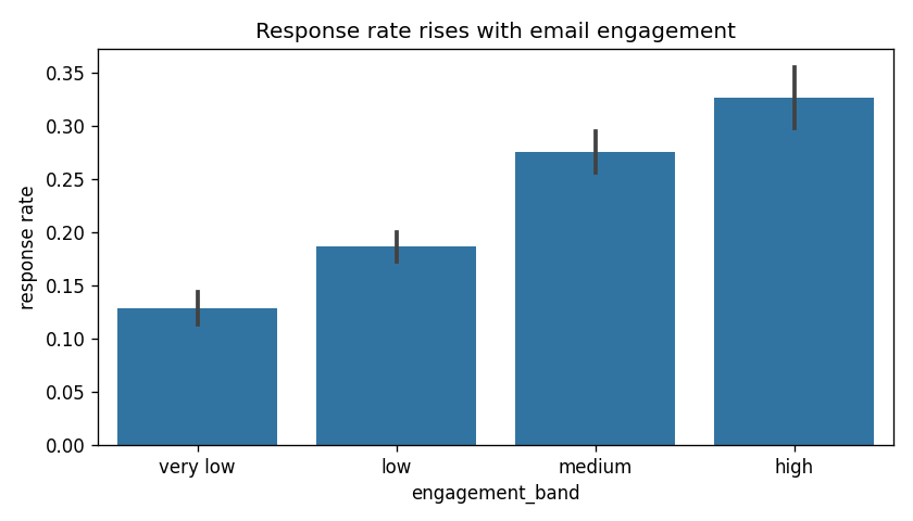
Phase 5 — Feature engineering and encoding
Two light domain features, then one-hot encode the three categorical columns. We keep this minimal because the focus is tuning, not feature engineering.
df["recent_buyer"] = (df["days_since_last_purchase"] < 30).astype(int)
df["engaged"] = (df["email_open_rate"] > 0.4).astype(int)

df = pd.get_dummies(df, columns=["channel", "segment", "region"], drop_first=True)
Phase 6 — Model selection and baseline
A stratified split preserves the 22% positive rate in both halves. The baseline is a Random Forest with default settings: the number every tuned model must beat.
X = df.drop(columns=["responded"])
y = df["responded"]

X_train, X_test, y_train, y_test = train_test_split(
    X, y, test_size=0.25, random_state=SEED, stratify=y)

baseline = RandomForestClassifier(random_state=SEED)
baseline.fit(X_train, y_train)
baseline_auc = roc_auc_score(y_test, baseline.predict_proba(X_test)[:, 1])
print("Baseline (default RandomForest) test ROC-AUC: {:.4f}".format(baseline_auc))
Baseline (default RandomForest) test ROC-AUC: 0.6929Phase 7 — Tuning
7.1 Manual search over one hyperparameter
The most basic tuning there is: loop over tree depth and record the 5-fold cross-validated AUC on the training data only.
for d in [3, 5, 8, 12, 20, None]:
    m = RandomForestClassifier(max_depth=d, n_estimators=100, random_state=SEED)
    cv_auc = cross_val_score(m, X_train, y_train, scoring="roc_auc", cv=5).mean()
    print(d, round(cv_auc, 4))
3 0.6677
5 0.6746
8 0.6784
12 0.6705
20 0.6643
None 0.66037.2 Learning curve over the number of trees
n_values = [10, 25, 50, 100, 200, 300]
aucs = []
for n in n_values:
    m = RandomForestClassifier(n_estimators=n, max_depth=8, random_state=SEED)
    aucs.append(cross_val_score(m, X_train, y_train, scoring="roc_auc", cv=5).mean())

plt.plot(n_values, aucs, marker="o")
plt.xlabel("n_estimators"); plt.ylabel("CV ROC-AUC")
plt.title("More trees help, then plateau")
plt.show()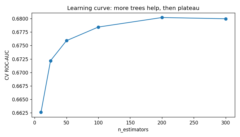
7.3 GridSearchCV — exhaustive over a small grid
rf_grid = {
    "n_estimators": [200],
    "max_depth": [6, 10, 16],
    "min_samples_leaf": [1, 5, 20],
    "max_features": ["sqrt", "log2"],
}
grid_rf = GridSearchCV(RandomForestClassifier(random_state=SEED),
                       rf_grid, scoring="roc_auc", cv=5, n_jobs=-1, refit=True)
grid_rf.fit(X_train, y_train)
print(round(grid_rf.best_score_, 4), grid_rf.best_params_)
0.6842 {'max_depth': 10, 'max_features': 'sqrt', 'min_samples_leaf': 20, 'n_estimators': 200}7.4 RandomizedSearchCV — sample a large space
Gradient boosting has a bigger, partly continuous space. Sampling 25 random combinations is far cheaper than exhausting it, and tends to find a strong region anyway.
gbm_space = {
    "n_estimators": [100, 200, 300, 400],
    "learning_rate": np.linspace(0.01, 0.3, 30),
    "max_depth": [2, 3, 4, 5],
    "min_samples_leaf": list(range(1, 40)),
    "subsample": [0.7, 0.8, 0.9, 1.0],
}
random_gbm = RandomizedSearchCV(GradientBoostingClassifier(random_state=SEED),
                                gbm_space, n_iter=25, scoring="roc_auc",
                                cv=5, n_jobs=-1, random_state=SEED, refit=True)
random_gbm.fit(X_train, y_train)
print(round(random_gbm.best_score_, 4), random_gbm.best_params_)
0.6925 {'subsample': 1.0, 'n_estimators': 400, 'min_samples_leaf': 20,
'max_depth': 2, 'learning_rate': 0.03}7.5 Coarse-to-fine — refine the winning region
best_lr = random_gbm.best_params_["learning_rate"]
best_depth = random_gbm.best_params_["max_depth"]

fine_grid = {
    "n_estimators": [random_gbm.best_params_["n_estimators"]],
    "learning_rate": [max(0.01, best_lr * 0.7), best_lr, best_lr * 1.3],
    "max_depth": sorted({max(2, best_depth - 1), best_depth, best_depth + 1}),
    "subsample": [random_gbm.best_params_["subsample"]],
    "min_samples_leaf": [random_gbm.best_params_["min_samples_leaf"]],
}
fine_gbm = GridSearchCV(GradientBoostingClassifier(random_state=SEED),
                        fine_grid, scoring="roc_auc", cv=5, n_jobs=-1, refit=True)
fine_gbm.fit(X_train, y_train)
print(round(fine_gbm.best_score_, 4), fine_gbm.best_params_)
0.6925 {'learning_rate': 0.03, 'max_depth': 2, 'min_samples_leaf': 20,
'n_estimators': 400, 'subsample': 1.0}Final evaluation — tuned vs default
Pick the search with the best cross-validated AUC, then judge it once on the held-out test set.
best = random_gbm.best_estimator_          # the random-search GBM won
tuned_proba = best.predict_proba(X_test)[:, 1]
tuned_pred = best.predict(X_test)

print("Default AUC : {:.4f}".format(baseline_auc))
print("Tuned AUC   : {:.4f}".format(roc_auc_score(y_test, tuned_proba)))
print(confusion_matrix(y_test, tuned_pred))
print(classification_report(y_test, tuned_pred))
Default AUC : 0.6929
Tuned AUC : 0.7239
[[1546 23]
[ 391 40]]
precision recall f1-score support
0 0.80 0.99 0.88 1569
1 0.63 0.09 0.16 431
accuracy 0.79 2000| Model | Test ROC-AUC |
|---|---|
| Default Random Forest (baseline) | 0.693 |
| Tuned Gradient Boosting | 0.724 |
| Improvement | +0.031 |
The tuned Gradient Boosting model reached a test ROC-AUC of 0.724, beating the default Random Forest’s 0.693 by a clean +0.031. Notice the honest lessons: tuning the Random Forest barely helped, switching model family is what moved the needle; coarse-to-fine confirmed the region rather than improving it; and recall at the default threshold is low, which is why we judge on ranking, not accuracy.
Phase 8 — Documentation and handoff
The campaign team works a ranked list, so we rank the test customers by predicted probability and report precision in the top 200, the slots a fixed budget can afford.
ranked = X_test.copy()
ranked["true_responded"] = y_test.values
ranked["response_probability"] = tuned_proba
ranked = ranked.sort_values("response_probability", ascending=False)

print("Precision@200: {:.1%}".format(ranked.head(200)["true_responded"].mean()))

import joblib
joblib.dump(best, "campaign_response_model.joblib")
Precision@200: 51.0%Precision@200 of 51% against a 21.5% base rate means the ranked list more than doubles the hit rate for a fixed budget, which is the result the business actually cares about. For the concepts behind every method used here, see the companion guide, Hyperparameter Tuning in Python.


[…] Hyperparameter Tuning, Start to Finish: A Code-Along […]
[…] Hyperparameter Tuning, Start to Finish: A Code-Along […]